Introduction/Background
Our group is interested in finding out what factors can be considered in detecting Type 2 diabetes. Diabetes is a condition that affects over 1 in 10 Americans, with almost 1 in 3 Americans at high risk of diabetes in the future [1].
Problem Definition
Diabetes is a medical condition in which a patient cannot make use of insulin and has low blood sugar levels as a result [2]. Currently, diabetes is typically diagnosed through either the A1C test, the FPG test, the OGTT, or the Random Plasma Glucose Test [3]. All tests aim to measure patients’ glucose levels in order to determine whether they have diabetes, prediabetes, or neither. A concern that follows these diagnoses arises from the fact that glucose level is a relatively volatile metric, and each test aims to combat this issue by varying the frequency, amount, and method of glucose level testing. All of these methods are still at risk of error and some require too much time and energy for the average person to utilize. Our group aims to fix this issue by providing an accurate metric for patients curious about their risk of diabetes in a timelier, more precise manner. By utilizing modern Machine Learning techniques, we hope to be able to develop an algorithm that inputs relevant patient information and outputs the likelihood that the given patient has diabetes. This will provide actionable help for the general population, as people with a greater likelihood metric will be more aware of the fact that further testing is absolutely necessary.
Data Collection
Data Source
Our dataset was accessed from a public Kaggle dataset collected from the National Institute of Diabetes and Digestive and Kidney Diseases. In order to constrain the data to avoid inaccurate assumptions, this dataset consists strictly of patients that are females, at least 21 years old, and of Pima Indian heritage. It includes the following information about each patient: number of pregnancies, glucose, blood pressure, skin thickness, insulin, BMI, a diabetes pedigree function value, age, and whether or not the patient ended up being diagnosed as diabetic.
Data Cleaning
A complication with this dataset is that it contained numerous entries in which one or more of the entries were invalid; that is, they contained 0 values in the context of a metric in which a value of 0 is inaccurate (blood sugar, skin thickness, etc.). In order to clean the data, we considered each of the following methods:
-
Dropping Rows Containing Invalid Entries
The issue with this method is that the dataset already only contained 768 entries, and applying this technique would have lowered our dataset size down to only 392 entries. -
Inserting the Average Value of the Metric into Entries with Invalid Values
This method, while sacrificing a bit of accuracy by picking the average value for an unknown value, solves the far more crucial issue of having a dataset too small in size. This method maintains the size of our original dataset.
Methods
Neural Network Classification
The supervised first method implemented in this project involved constructing a rudimentary neural network in order to predict whether or not a given patient has diabetes, given a set of relevant medical information about the patient. We are thus left with a large list of hyperparameters to optimize; we will discuss this optimization in the Results and Discussion section below.
Feature Reduction Using PCA
In order to combat overfitting and introduce the number of features as a hyperparameter that we will fine tune, we will implement PCA as our feature reduction algorithm of choice. We will discuss the optimal number of features to consider in the Results and Discussion section below.
Training Validation Test Split
It is important to mention that we utilized an 80% training data, 10% validation data, and 10% test data split in order to train our neural network. This means that we utilize the vast majority of our data in order to train our model, but we save 10% of it in order to validate how our model performs compared to a dataset other than our training data. Finally, we utilize the remaining 10% of the data in order to test to see how our validated model performs on a “random” dataset.
For methods in which no validation data is needed, we went with an 80% training data 20% test data split for the sake of consistency and the ability to compare between methods that require validation data and methods that don’t.
Naive Bayes Classification
The second supervised method that our group utilized in this project is Naive bayes classification. Although Naive Bayes operates on the assumption that all of the features are independent, which may not be true for this data, our group decided to test how well it would perform given our data. We implemented the Gaussian variation of Naive Bayes provided through the SkLearn framework.
Random Forest Classification
The third supervised method that our group implemented was the random forest classification method. This method utilizes decision trees to classify data, and has three hyperparameters: the number of estimators for the forest, the maximum depth of the forest, and the percentage of the maximum number of features utilized. We will discuss how we optimized these hyperparameters in the results and discussion section.
Perceptron Algorithm Classification
Our final supervised method for this project is the perceptron algorithm. This method was mainly implemented to see if our data was linearly separable. This method was sort of a trial method to understand what kind of data we were dealing with.
Results and Discussion
Neural Network Classification
In order to fine tune a neural network and all of its hyperparameters, a base is laid down and the hyperparameters are identified first. As previously mentioned, PCA has enabled us to include the number of features of our dataset as a hyperparameter. We will identify the rest of the hyperparameters by constructing a barebones neural network on the dataset using the aforementioned average method.
In order to implement this neural network, we utilized a TensorFlow Tutorial that walked us through how to build a rudimentary neural network in TensorFlow. The tutorial explained the construction of a neural network that predicted whether or not a pet would be adopted given a set of characteristics about the pet.
In order to prepare our dataset for neural network processing, we must first turn our dataframe into a TensorFlow dataset. This involves a) dropping the column of our dataframe that tells us whether or not the given patient ended up being diagnosed with diabetes and b) grouping the rows into groups of data called batches, with the size of each batch being a hyperparameter that we will optimize below. To begin with, we chose a batch size of 5.
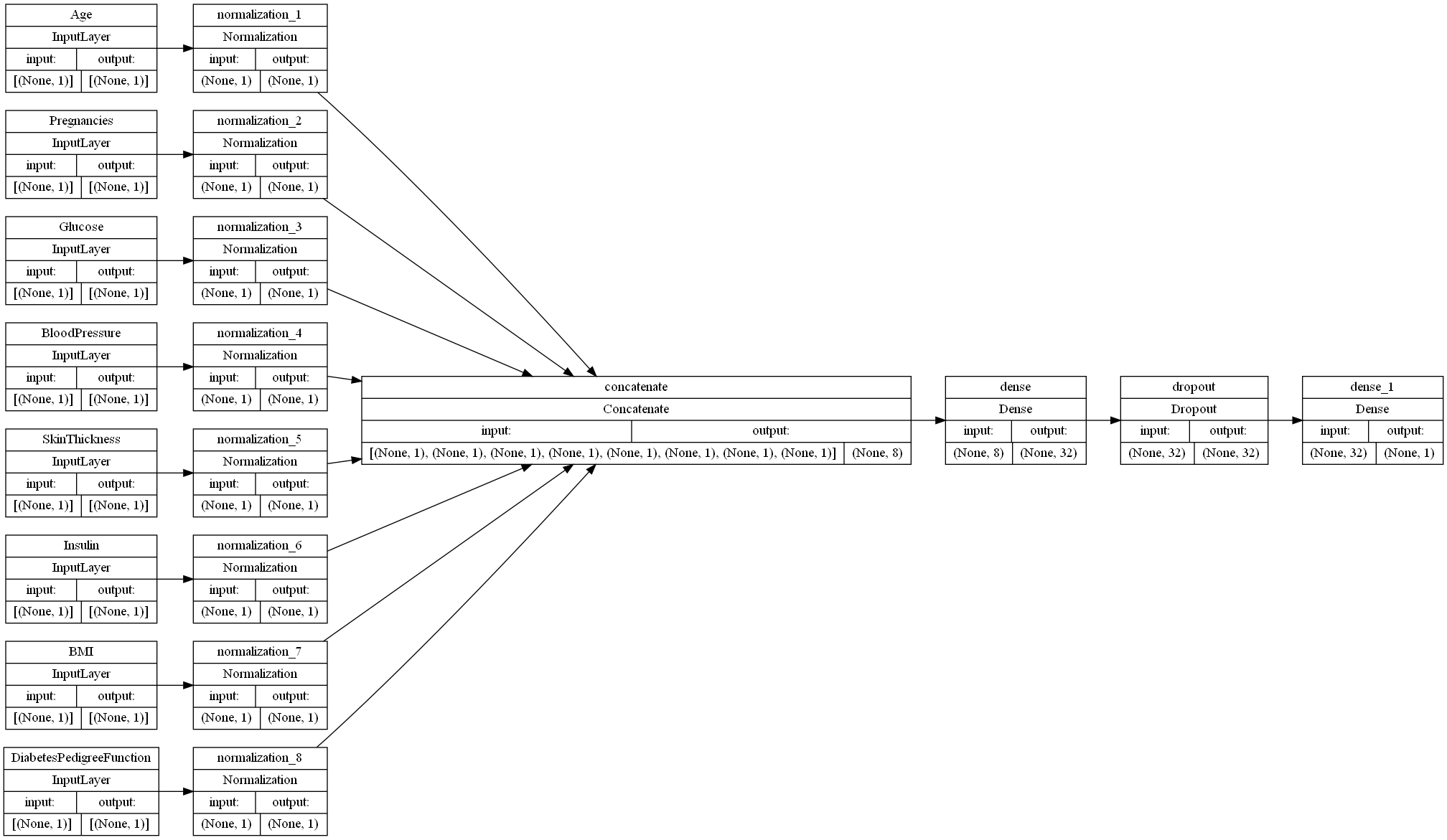
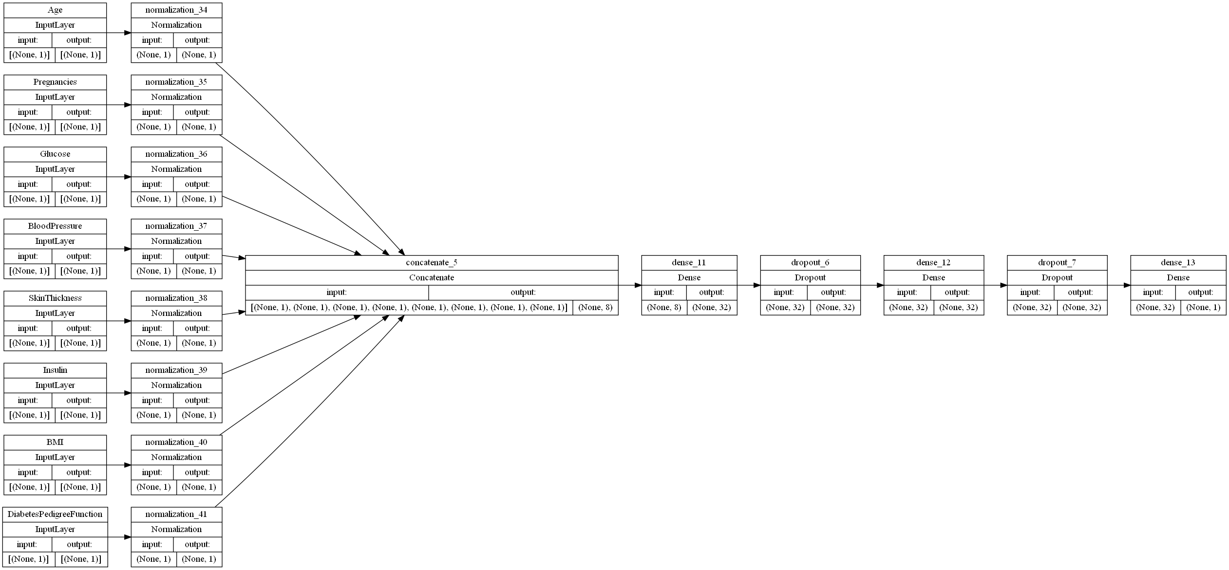
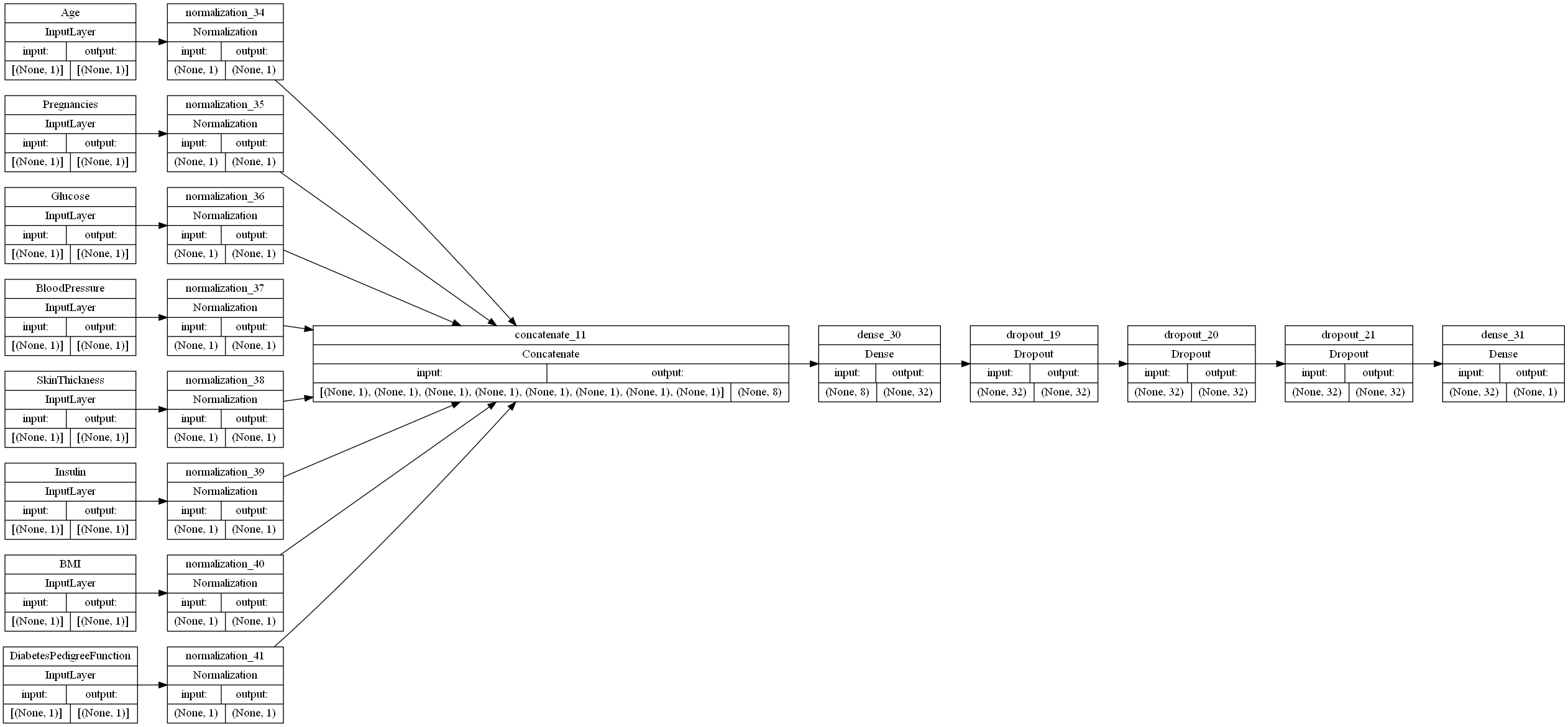
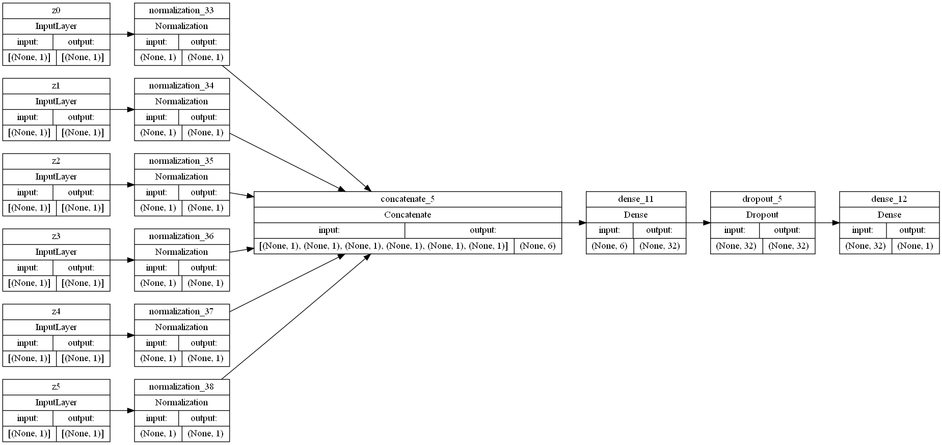
The neural network begins with a preprocessing layer for the data. Keras provides numerous options for preprocessing dataset features, but, since all of our features are integer, non-categorical features, we applied a feature-wise normalization to each of our input features.
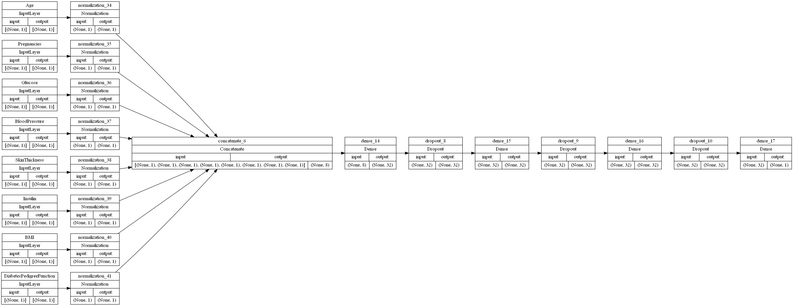
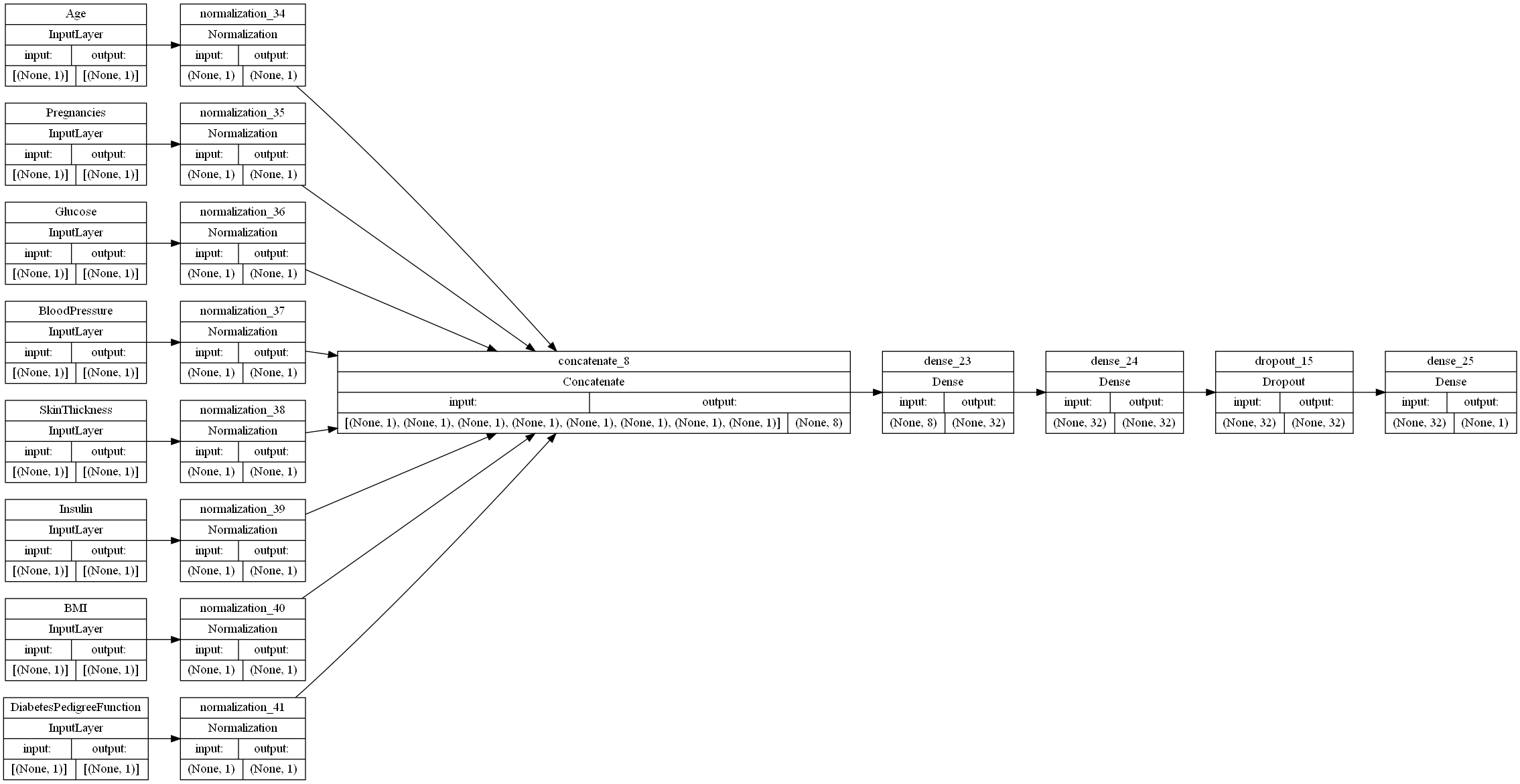
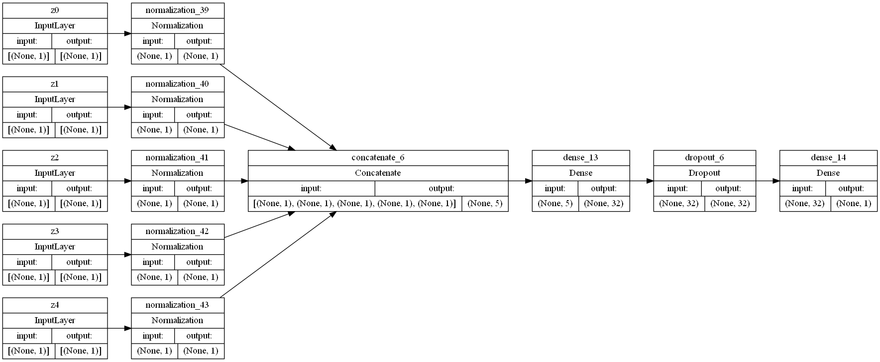
Once our features are encoded, we are ready to apply some Fully Connected (FC) layers to our mode, which are referred to as “Dense” layers in TensorFlow. The number and types of layers that we have are hyperparameters, so we will begin with two layers to lay a base for optimization. Our first layer is a Dense layer consisting of 32 perceptrons, each of which perform Relu on our inputs. Our second layer is a Dropout layer, which sets a portion of our inputs to 0 at a given frequency value ranging from 0 to 1. For the sake of simplicity, we chose 0.5 for our frequency value.
The initial neural network configuration is shown below:
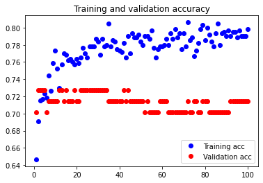
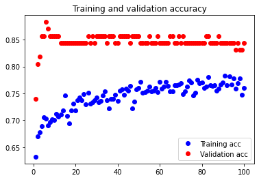
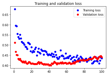
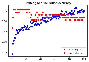
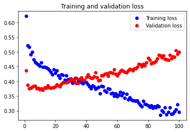
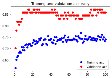
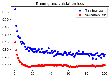
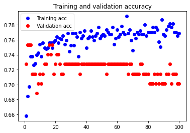
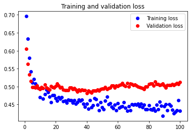
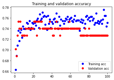
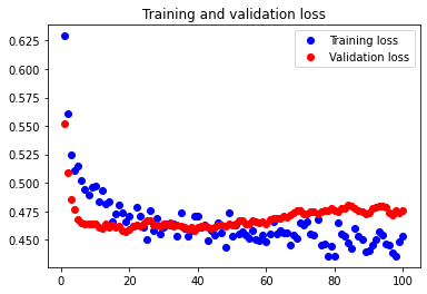
The initial accuracy and loss graphs for the training set vs the validation set are shown below:
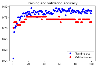
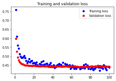
This model resulted in a test accuracy of 77.922%. Our initial results are quite strong and have very small amounts of overfitting, but we will attempt to optimize our model further through fine tuning our hyperparameters.
Optimizing batch size
Batch size of 3
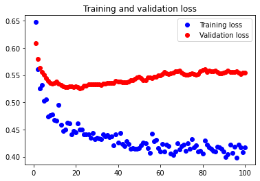
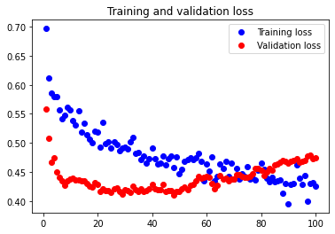
Beginning with a batch size of 3, we see that it is slightly overfitted compared to the network of batch size 5 as shown below.
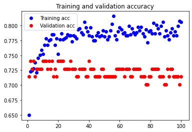
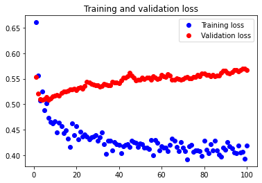
The test accuracy is 76.623%, which is slightly smaller than the test accuracy value for batch size 5. We can thus see that batch size 5 is better than batch size 3 in this case.
Batch size of 7
When we set batch size to 7, we see that it is again slightly overfitted compared to batch size 5.
The test accuracy is 76.623% again, which is slightly smaller than the test accuracy value for batch size 5. Batch size 5 is thus better than batch size 7 in this case.
Optimizing FC layers
In this section, we attempted to optimize the amount and type of FC layers our neural network has in order to maximize our test dataset accuracy.
Doubling our current layout
The first thing we tested was doubling our current layout. Although this would, in theory, increase overfitting, doubling the Dropout layer in addition might combat this overfitting and lead to an increase in both accuracies.
The test accuracy was 75.235%. As we see in this case, the attempt to reduce underfitting failed. Doubling our current configuration only increased the amount of overfitting in our neural network.
Tripling our current layout
In order to ensure that the previous results were not anecdotal, we tried tripling our current layout to see if we could increase all of our dataset accuracies.
The test accuracy was 74.026%. Again, the results show that multiplying our current configuration only increases overfitting.
Adding an extra dense layer
Though adding non-dropout FC layers is meant to reduce underfitting and increase overfitting, we tried adding an extra Dense layer to see if this theoretical statement held true in practice.
The test accuracy was 71.429%. The theoretical statement that adding an extra Dense layer only increased the amount of overfitting in our neural network thus holds true.
Adding two extra dropout layers
In order to decrease overfitting, we tried adding two Dropout layers with dropout frequencies of 0.25, so as to avoid zeroing out too much of the data.
The test accuracy was 74.026%. As we see here, our attempt to decrease overfitting led to an underfitted model. Although it is not shown, we attempted adding only one Dropout layer, and underfitting occurred again.
FC Layer conclusion
The results are unexpected for this hyperparameter tuning, but we have determined that the best layer configuration that we have found so far is the initial configuration with 1 Dense layer consisting of 32 perceptrons and 1 Dropout layer with a dropout frequency of 0.5. Further optimization must be done in the next project iteration to find a better configuration that reduces both overfitting and underfitting in our model.
Optimizing number of features utilizing PCA
In order to vary the number of features in our data utilizing PCA, we adjusted the retained variance of the data until we generated an output with the desired number of features.
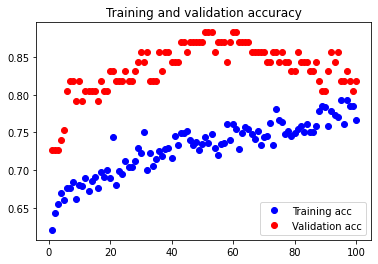
Considering 7 features
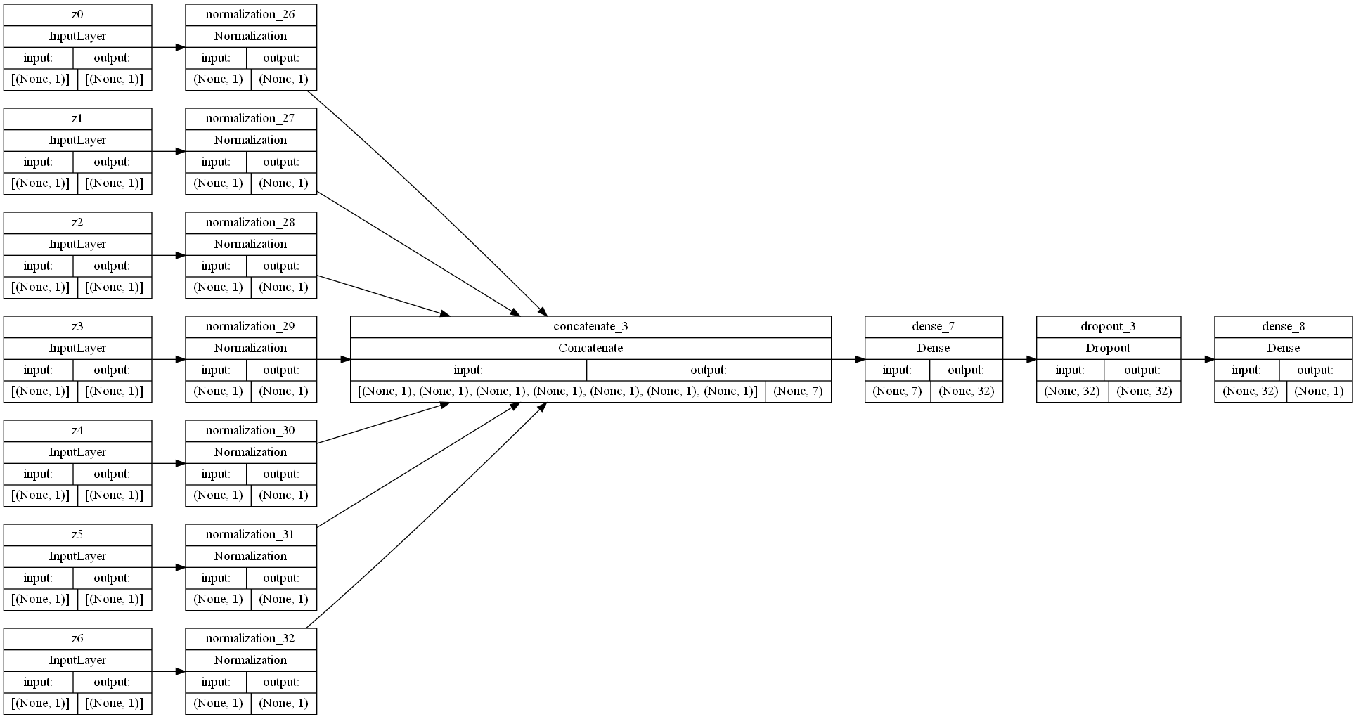
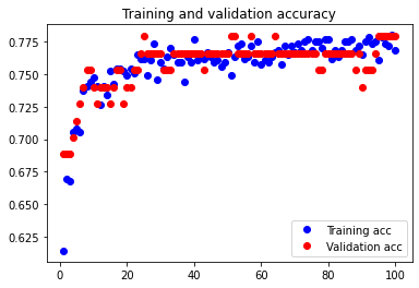
Here, we considered 7 features to determine whether considering fewer features would increase our test dataset accuracy. This would, in theory, increase our test accuracy by reducing overfitting.
The test accuracy was 79.221%. As we can see, considering 7 features works better than our initial configuration, so feature reduction does as expected. It reduced the amount of overfitting.
Considering 6 features
In order to see whether further reducing the number of features in our dataset would help combat overfitting to an even greater degree, we attempted considering 6 features.
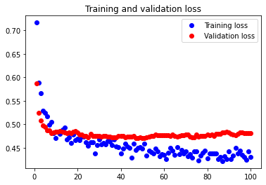
The test accuracy was 77.922%. This accuracy is worse than the accuracy achieved from considering 7 features, and there appears to be an extremely small amount of underfitting occurring.
Considering 5 features
To ensure that reducing the number of features in our dataset would result in more underfitting, we attempted considering only 5 features.
The test accuracy was 67.532%. Although there unexpectedly appears to be overfitting occurring, it is clear that reducing our features even further leads to volatile results and a decrease in test accuracy.
Feature reduction conclusion
Through a slight variation of the elbow method, we have determined that considering 7 features produces the optimal results for our neural network. Though a full implementation of the elbow method or another parameter validation method must be completed in the next project iteration, this conclusion will suffice for now.
Neural Network Conclusion
We have thus concluded that a simple neural network with 1 Dense layer containing 32 perceptrons and 1 Dropout layer with a dropout rate of 0.5 is the ideal configuration for our neural network. Additionally, a batch size of 5 and a feature reduction to 7 features is the ideal data transformation for this neural network. This configuration enabled us to reach a test set accuracy of 79.221%.
Naive Bayes Classification
Since we utilized the Gaussian Naive Bayes method provided through the SkLearn framework, there were no hyperparameters for this particular method. Additionally, due to the nature of Naive Bayes, the only metric provided for this metric is accuracy. We analyzed only test dataset accuracy in this method. As an additional hypermeter and an attempt to optimize Naive Bayes, we attempted to utilize PCA in order to add the number of features considered as a hyperparameter.
All features considered
When we run Gaussian Naive Bayes with all features considered, we get the following test dataset accuracy:
This accuracy is quite good, but it is still worse than the accuracy achieved with our optimized neural network. Perhaps we can do better by reducing the number of features.
7 features considered
When we run Gaussian Naive Bayes with only 7 features considered, we get the following test dataset accuracy:
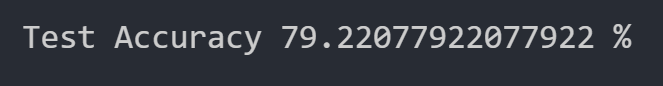
This accuracy is better than the one achieved when we considered all features, and it is actually eerily the exact same accuracy achieved with our optimized neural network. We will continue to reduce the features to see if we can get our accuracy any higher.
6 features considered
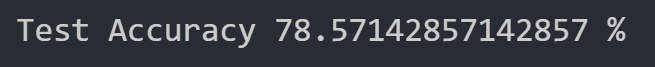
Here is the test dataset accuracy when we run Gaussian Bayes with only 6 features considered:
This is the same accuracy achieved when we consider all features. We will try to reduce the number of features further to ensure that 7 features is the optimal number of features to consider.
5 features considered
Here is the test dataset accuracy when we run Gaussian Bayes with only 5 features considered:

We can see that reducing our features produces a downward trend in accuracy, so we have determined that considering 7 features gives us the optimal accuracy with Gaussian Naive Bayes.
Naive Bayes Conclusion
We have thus concluded that considering 7 features when running Gaussian Naive Bayes produces the optimal test dataset accuracy, and we achieved an accuracy of 79.221% with this method.
Random Forest Classification
As we mentioned previously, for the random forest classification method, we have three hyperparameters inherent with the method: the number of estimators for the forest, the maximum depth of the forest, and the percentage of the maximum number of features utilized. We will begin with considering the cleaned dataset and finding the optimal combination of values of the three hyperparameters. For the number of estimators for the forest, we can consider values between 3-15, for the maximum depth of the forest, we can consider values between 5 and 15, and for the maximum number of features, we can consider values between 0.6-1.0.
Utilizing Randomized Search Cross Validation
In order to optimize the hyperparameters of the random forest, we utilized the RandomizedSearchCV from the SkLearn framework. It generates a large grid with tiles containing a random selection of hyperparameter values. The algorithm then selects a set of random tiles and picks the tile with the largest test accuracy value in order to determine the optimal hyperparameter values. The output of the cross validation algorithm is as shown below:
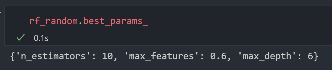
We then created a random forest using the discovered hyperparameters.
An example tree from the forest we produced is given below:
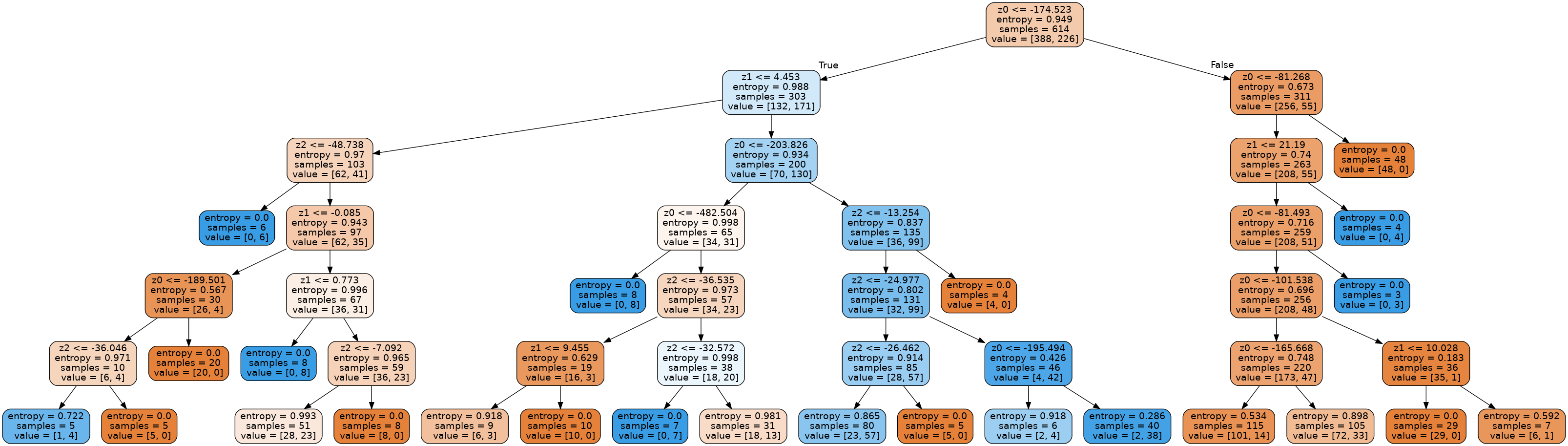
We were able to get the following test dataset accuracy with our random forest:

Including PCA
We then attempted to optimize our model even further by considering fewer features through PCA.
Considering 7 features
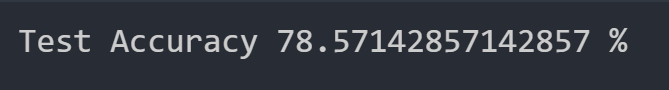
When we consider only 7 features for our random forest model, we get the following test dataset accuracy:
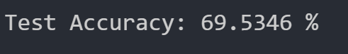
This accuracy is no better than the accuracy achieved when we consider all the features, but we will attempt to consider one less feature to see if there’s any sort of pattern for considering less features.
Considering 6 features
When we consider only 6 features for our random forest model, we get the following test dataset accuracy:
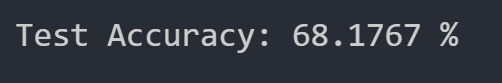
This accuracy is even worse than the accuracy achieved when considering 7 features, so we will stop our hyperparameter optimization here and conclude that considering all of the features is best for this random forest algorithm.
Random Forest Conclusion
We have thus concluded that the best test dataset accuracy we can achieve with the random forest algorithm is 70.464%. This accuracy is relatively low compared to our other methods.
Perceptron Algorithm Classification
For our perceptron algorithm, we utilized the built in SkLearn linear perceptron model and thus have no hyperparameters. We ran this algorithm simply to see how well high our test accuracy would be for this function in order to determine whether our data is at least close to being linearly separable. Upon running the perceptron algorithm the first time, we got the following test dataset accuracy:

Since our accuracy is so low straight off the bat, we will not attempt to optimize it during PCA and conclude that our data is not very linearly separable; thus, the perceptron algorithm is a poor choice for this dataset.
Conclusions
We have thus concluded that the highest test accuracy we can achieve for our dataset occurs when we utilize a Keras Neural Network Model with PCA or Gaussian Naive Bayes with PCA. The highest test dataset accuracy was 79.221%, and we achieved this accuracy with both the Neural Network and the Naive Bayes approach. Both of these approaches proved to be far more effective for our dataset than the random forest algorithm and especially the perceptron algorithm.
Timeline
Nov 26: Implement the second and third supervised methods
Nov 30: Finish supervised method implementation
Dec 5: Final project completed
Dec 7: Turn in final project
References
[1]: https://www.cdc.gov/diabetes/library/features/diabetes-stat-report.html
[2]: https://www.cdc.gov/diabetes/basics/diabetes.html
[3]: https://www.diabetes.org/a1c/diagnosis